📔 Notes On: Scaled Dot-Product Attention
 Read on Substack
October 14, 2024
Attention is here to stay. For anyone at least remotely interested in deep learning, including myself, it’s valuable to revisit its foundational principles from time to tome. Let’s dive in!
✅ What I’d like to cover in this post is:
- A brief introduction to scaled dot-product attention, hereafter referred to as attention.
- A small experiment in which I visualize the query and key vector space
🚫 What I do not want to cover?
- An architecture of a Transformer (Attention Is All you Need)
- The history of attention and all its variations.
📖 Scaled Dot-Product Attention — The Theory
In general, attention in the context of natural language processing offers a different approach to ‘sharing’ information between individual tokens being processed by a model. While it’s true that the Transformer model, which heavily relies on the attention mechanism, was initially introduced to solve the problem of language translation, nowadays we also encounter Transformer based models processing images, where a token represents not a part of a sentence but a part of an image. In the end, it’s all just numbers.
In comparison to RNNs or models like Mamba where the information between tokens is shared through a hidden state that requires some compression of previously seen tokens, the attention mechanism provides the models with the ability to take a look at the input sequence at once and decide which information should be shared between the tokens in order to successfully proceed in the computation that the model was trained to do.
The ability to at once take a look at an uncompressed version of the processed data gives the attention its power. However, nothing comes without a cost and even attention has its price. There are two major challenges associated with attention:
-
scalability — As we will show later, attention scores are stored in a matrix that grows quadratically with the length of the input sequence. Thanks to this fact we have to put the computational complexity of attention based models to O(n²).
-
fixed-sized context — There is a fixed upper limit to how long sequences can be processed at once by attention-based models. Simply put, the larger the context, the longer conversations you can have with your favorite LLM without the model forgetting some information along the way.
Now, let’s take a look at the core of the attention mechanism. Here it is. Scaled dot-product attention:

(Equation 1) scaled dot-product attention
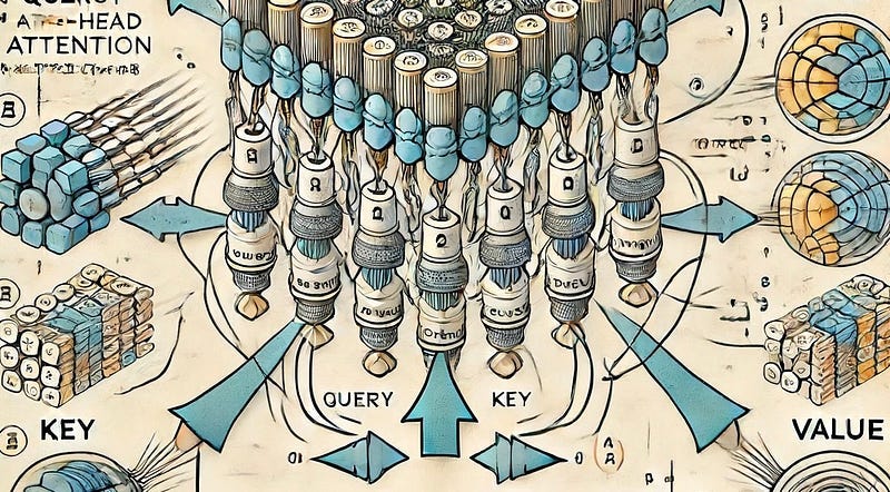
I suggest we digest this formula bit by bit. First, let’s investigate the three input matrices: Q (query), K (key), V (value). Each matrix contains vectors, while each vector represents one word from the input sentence. For demonstration purposes, we can use the following sentence: “I was watching the door when it opened.”

(Picture 1) A picture depicting a matrix containing vectors representing words from our sample sentence, before it is processed by the scaled dot product attention block in a Transformer. Before the matrix reaches the attention block, it undergoes three separate linear transformations. The linear transformations output three matrices Q (query), K (key), V (value).
As the vectors representing the words are passing through the model, before they reach the attention part, they get passed through linear transformation that puts on the vectors different meaning (Picture 1). For now, it should be enough to know that the following applies for the vectors in the individual matrices:
-
❓Q (query): Vectors in this matrix exist in the query space. Their position in this space indicates what information the vectors are seeking. From our example, the word “watching” (a verb) might be looking for “door” (a noun) at a certain depth in the model.
-
🔑 K (key): Vectors in this matrix exist in the key space. Their position tells what information the vectors provide. Again, from our example, a vector representing word “door” might be placed in such a subspace of the key space which indicates that it is a noun.
-
🔢 V (value): Vectors in this matrix exist in the value space. This is the actual value the vectors are offering. This value is passed between the vectors depending on how strong the match is between the supply (keys) and demand (queries).
The core of the attention mechanism lies in the multiplication of the Q and K matrices. It doesn’t take much imagination to notice that the higher the dot product between individual vectors from the Q and K matrices, the higher the resulting attention score for the given pair. This means that when the supply (Q) meets the demand (K), the resulting attention score is higher.
The resulting product of the Q and K matrices is divided by sqrt(d_k). The idea behind this division is to scale down the vectors because, as the number of dimensions of the input vectors increases, so does the output of the dot product. This scaling might lead to the vanishing gradient problem, which is connected to the softmax function.

(Picture 2) An example of a matrix containing the computed attention scores. These particular scores ensure the exchange of information between the vectors representing the words “watching” and “door”. This is the state of the attention matrix prior to the multiplication with the matrix V.
Finally, we pass the matrix through the softmax function, which yields a matrix where the value at index i, j represents how much attention a word at index i is paying to the word at index j in our sample sentence: “I was watching the door when it opened.” In other words, it indicates how much information should be transferred from the token at index j to the token at index i (Picutre 2).

(Equation 2) The final vector representing word “watching” which leaves the attention block is calculated as a weighted average of vectors from matrix V. The weights are taken from the attention matrix.
By multiplying the matrix with the V matrix we reach the point where the vectors exchange the information between each other (Equation 2).
👀 Visualizing Attention
Let’s take a look at attention in practice. In this small experiment, we’ll examine the actual attention scores calculated inside a BERT model. This model is based on the encoder component of the original Transformer from the Attention Is All You Need paper. The authors aimed to create a generic pre-trained model that can later be fine-tuned for specific language tasks. For our experiment, it is important to note that the model was trained on two specific tasks:
- Replacing the
[MASK]token with a word that best fits the given context. For example, “I[MASK]a person.” → “I am a person.” - Given two sentences, deciding whether sentence B follows sentence A. For example, “I am going to the supermarket. I would like to buy apples.” → YES, and “I am going to the supermarket. And that is how I met your mother.” → NO)
We will leverage the fact that the model was trained on the task of replacing the
[MASK] token with the word that best fits the sentence. Our experiment consists
of three main parts:
- Passing sentence “I was watching the
[MASK]when it opened.” to a pre-trained BERT model. - Investigating the calculated attention scores.
- Using t-SNE dimensionality reduction technique to display vectors from the query and key spaces.
If anyone is interested in the code, you can find it here. We’re using the
bert-base-uncased5 model. For the rest of this discussion, we will focus on
the values calculated in the layer with index 3 and head with index 11. The main
reason for focusing on this particular layer and head is that it contains
attention scores that are relatively easy for us humans to interpret.
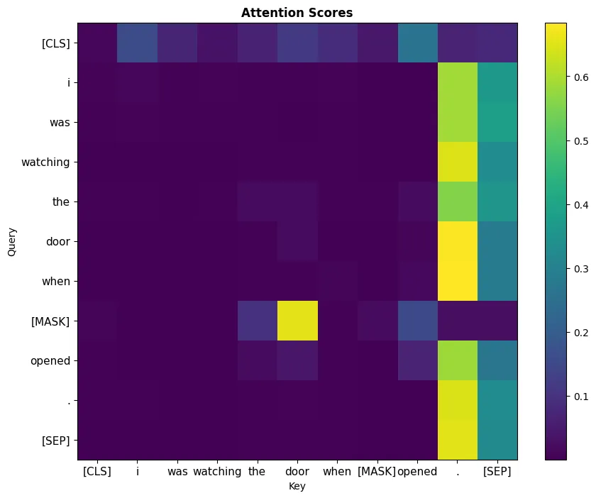
(Picture 3) Values calculated in the bert-base-uncased model
(layer index = 3, head index = 11) when processing the “I was watching the
door when [MASK] opened.” sentence. Notice the high attention score between
the vector representing the [MASK] token and the door token.
We can see that in the layer and head under investigation, there is a high
attention value for the [MASK] and “door” token pair (Picture 3). Most of
the time, it is hard to put meaning on the values calculated during
the computation of attention; however, in this particular case, we see something
that one might expect.
Logically, we can expect with high probability that there needs to be a certain
exchange of information between the door and the [MASK] token somewhere during
the processing of the sentence. The reason for this is that [MASK] should be
replaced with ‘it’, which clearly references the “door” in the sentence.
Now, let’s use the t-SNE dimensionality reduction technique to investigate the
location of the query and key vectors in the Query-Key vector space. We will use
the cosine distance as a distance metric for the dimensionality reduction
algorithm to showcase the closeness of the query vector representing [MASK]
and key vector representing “door”.
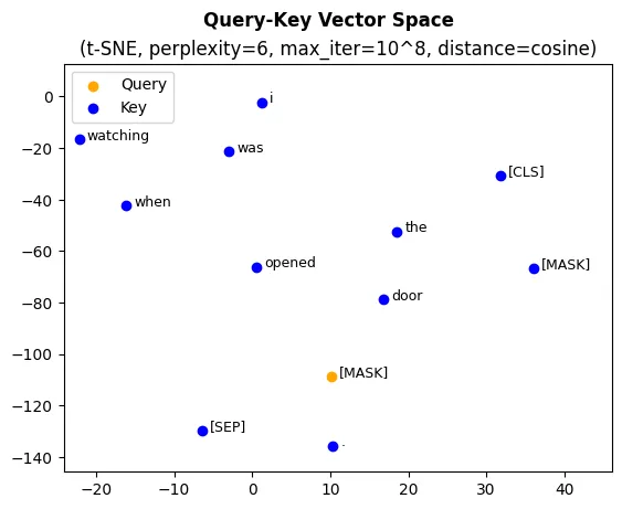
(Picture 4) A graph of the Query-Key vector space reduced to two
dimensions using the t-SNE dimensionality reduction method (number of iterations = 10⁸,
perplexity = 5, distance = cosine). The graph demonstrates the closeness
between the [MASK] vector and the rest of the Key vectors.
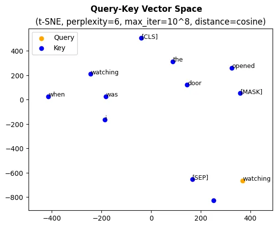
(Picture 5) A graph of the Query-Key vector space
reduced to two dimensions using the t-SNE dimensionality reduction method
(number of iterations = 1⁰⁸, perplexity = 5, distance = cosine).
The graph demonstrates the distance between the vector representing the
“watching” token and the rest of the Key vectors.
In Pictures 5 and 6, you can see that the vector representing token [MASK]
is significantly closer to the token “door” than, for example, the query vector
representing word “watching”. This closeness ensures the high attention score
for the given pair of tokens, facilitating a successful exchange of the
information between them.
You can now imagine, at a high level, what is happening during the training of the Transformer model. TL;DR: The model tries to find such weights which transform the vectors incoming into the attention block in such a way that:
-
Query and key vectors that need to exchange information (
[MASK]and “door” in our example) for successful task performance are positioned in such a way that their dot product is high. -
On the other hand, vectors that should exchange as little information as possible are positioned in such a way that their dot product is low (
[MASK]and “watching in our example).